Trajectory Workflow
Direct command workflow for trajectory analyses.
This module implements CLI workflow orchestration for its command family, including argument parsing, request construction, execution dispatch, and result presentation handoff.
Usage context
- Command routing: Resolve CLI aliases and normalized command names.
- Task execution: Build request objects and invoke registered tasks.
- Output handling: Forward results to table, plot, export, or report flows.
Command: msd
Compute time-origin averaged mean-squared displacement (MSD) for selected atoms.
The output is averaged over selected atoms and all valid time origins, giving MSD vs lag time.
Examples
  1. Plot MSD for selected atom ids:
   reaxkit get_msd --atom-ids 1 2 3 --max-lag 500 --delta-t-ps 0.25 --plot single

  2. Save oxygen-only MSD vs lag time:
   reaxkit get_msd --atom-types O --max-lag 800 --delta-t-ps 1.0 --save msd_oxygen.png

  3. Export MSD using selected frames:
   reaxkit get_msd --atom-ids 5 --frames 0:1000:10 --max-lag 80 --export msd_atom5.csv
Arguments
Scientific choices
| Flag |
Required |
Default |
Help |
Choices |
--frames |
No |
|
Frame selector syntax. Example: --frames 0:20:2, which selects frames 0,2,4,...,20. |
|
--every |
No |
1 |
Frame stride. Example: --every 5, which keeps every fifth selected frame. |
|
--atom-ids |
No |
|
1-based atom ids. Example: --atom-ids 1 2 3, which restricts MSD to those atoms. |
|
--atom-types |
No |
|
Element symbols to include. Example: --atom-types O, which computes MSD for oxygen atoms only. |
|
--dims |
No |
x, y, z |
Coordinate dimensions to include. Example: --dims x y, which computes MSD using in-plane displacement. |
|
--max-lag |
No |
|
Maximum lag in number of selected frames. Example: --max-lag 800, which computes MSD from lag 0 to lag 799. |
|
--delta-t-ps |
No |
1.0 |
Time between selected trajectory frames in ps. Example: --delta-t-ps 0.25, which reports lag time in ps. |
|
--unwrap, --no-unwrap |
No |
True |
Unwrap coordinates across periodic boundaries when cell data exists. Example: --no-unwrap, which keeps wrapped coordinates. |
|
| Flag |
Required |
Default |
Help |
Choices |
--engine |
No |
|
Engine override. Example: --engine reaxff, which applies ReaxFF-specific trajectory loading behavior. |
reaxff, ams, lammps |
--run-dir, --dir |
No |
. |
Run directory (fallback for detection). Example: --run-dir runs/job1, which sets backup path for file discovery. |
|
--xmolout, --file |
No |
|
Trajectory file path. Example: --xmolout runs/job1/xmolout, which provides coordinate trajectory input. |
|
Outputs and plots
| Flag |
Required |
Default |
Help |
Choices |
--plot |
No |
|
Render a plot. Example: --plot single, which creates one combined figure. |
single, subplot |
--show |
No |
False |
Show the generated plot window. Example: --show, which opens the figure interactively. |
|
--save |
No |
|
Save the generated plot to a file path. Example: --save msd.png, which writes the figure image to disk. |
|
--export |
No |
|
Write the result table to CSV. Example: --export rdf.csv, which saves tabular analysis output. |
|
--grid |
No |
|
Subplot grid like 2x2 or 2*2. Example: --grid 2x2, which arranges subplot panels in a 2-by-2 layout. |
|
--xaxis |
No |
frame |
Quantity on x-axis. Example: --xaxis time, which uses converted physical time when available. |
iter, frame, time |
--detail-format |
No |
|
Optional detail format (default: Parquet; legacy: CSV). |
parquet, csv |
Execution
| Flag |
Required |
Default |
Help |
Choices |
--execution |
No |
auto |
Execution backend; unsupported backends fall back to serial with a logged reason. |
auto, serial, threads, processes |
--workers |
No |
0 |
Frame workers: auto or N (default: auto). |
|
--chunk-size |
No |
0 |
Maximum in-flight frames: auto or N. |
|
Storage and cache
| Flag |
Required |
Default |
Help |
Choices |
--run-id |
No |
|
Run identifier for run-scoped layout. Example: --run-id run_91ac0e, which reuses that run identifier. |
|
--project-root |
No |
reaxkit_workspace |
Project root that contains inputs/, data/, analysis/, etc. Example: --project-root ./workspace, which stores run artifacts there. |
|
--analysis-id |
No |
|
Optional analysis artifact id; defaults to run id. Example: --analysis-id comparison-a, which names the analysis artifact explicitly. |
|
--input-cache, --no-input-cache |
No |
True |
Reuse parsed input frames across commands (default: enabled; use --no-input-cache to force source reads for reproducibility checks or benchmarks). Example: --no-input-cache, which reloads frames from their source files. |
|
--frame-cache-max-gb |
No |
10.0 |
Maximum workspace frame-cache size in GiB (default: 10; use 0 for unlimited). Example: --frame-cache-max-gb 20, which caps cached frames at 20 GiB. |
|
--output-profile |
No |
standard |
Select the shared artifact policy. Standard writes declared default outputs; minimal keeps core tables; full and legacy include optional details. Default: standard. Example: --output-profile full, which includes declared optional detail tables. |
minimal, standard, full, legacy |
Diagnostics and compatibility
| Flag |
Required |
Default |
Help |
Choices |
-h, --help |
No |
|
show this help message and exit |
|
--help-all, --all-flags |
No |
|
Show every option, grouped by purpose. |
|
--log |
No |
quiet |
Logging level. Example: --log verbose, which prints more runtime details. |
verbose, quiet |
Command: get_msd
Compute time-origin averaged mean-squared displacement (MSD) for selected atoms.
The output is averaged over selected atoms and all valid time origins, giving MSD vs lag time.
Examples
  1. Plot MSD for selected atom ids:
   reaxkit get_msd --atom-ids 1 2 3 --max-lag 500 --delta-t-ps 0.25 --plot single

  2. Save oxygen-only MSD vs lag time:
   reaxkit get_msd --atom-types O --max-lag 800 --delta-t-ps 1.0 --save msd_oxygen.png

  3. Export MSD using selected frames:
   reaxkit get_msd --atom-ids 5 --frames 0:1000:10 --max-lag 80 --export msd_atom5.csv
Arguments
Scientific choices
| Flag |
Required |
Default |
Help |
Choices |
--frames |
No |
|
Frame selector syntax. Example: --frames 0:20:2, which selects frames 0,2,4,...,20. |
|
--every |
No |
1 |
Frame stride. Example: --every 5, which keeps every fifth selected frame. |
|
--atom-ids |
No |
|
1-based atom ids. Example: --atom-ids 1 2 3, which restricts MSD to those atoms. |
|
--atom-types |
No |
|
Element symbols to include. Example: --atom-types O, which computes MSD for oxygen atoms only. |
|
--dims |
No |
x, y, z |
Coordinate dimensions to include. Example: --dims x y, which computes MSD using in-plane displacement. |
|
--max-lag |
No |
|
Maximum lag in number of selected frames. Example: --max-lag 800, which computes MSD from lag 0 to lag 799. |
|
--delta-t-ps |
No |
1.0 |
Time between selected trajectory frames in ps. Example: --delta-t-ps 0.25, which reports lag time in ps. |
|
--unwrap, --no-unwrap |
No |
True |
Unwrap coordinates across periodic boundaries when cell data exists. Example: --no-unwrap, which keeps wrapped coordinates. |
|
| Flag |
Required |
Default |
Help |
Choices |
--engine |
No |
|
Engine override. Example: --engine reaxff, which applies ReaxFF-specific trajectory loading behavior. |
reaxff, ams, lammps |
--run-dir, --dir |
No |
. |
Run directory (fallback for detection). Example: --run-dir runs/job1, which sets backup path for file discovery. |
|
--xmolout, --file |
No |
|
Trajectory file path. Example: --xmolout runs/job1/xmolout, which provides coordinate trajectory input. |
|
Outputs and plots
| Flag |
Required |
Default |
Help |
Choices |
--plot |
No |
|
Render a plot. Example: --plot single, which creates one combined figure. |
single, subplot |
--show |
No |
False |
Show the generated plot window. Example: --show, which opens the figure interactively. |
|
--save |
No |
|
Save the generated plot to a file path. Example: --save msd.png, which writes the figure image to disk. |
|
--export |
No |
|
Write the result table to CSV. Example: --export rdf.csv, which saves tabular analysis output. |
|
--grid |
No |
|
Subplot grid like 2x2 or 2*2. Example: --grid 2x2, which arranges subplot panels in a 2-by-2 layout. |
|
--xaxis |
No |
frame |
Quantity on x-axis. Example: --xaxis time, which uses converted physical time when available. |
iter, frame, time |
--detail-format |
No |
|
Optional detail format (default: Parquet; legacy: CSV). |
parquet, csv |
Execution
| Flag |
Required |
Default |
Help |
Choices |
--execution |
No |
auto |
Execution backend; unsupported backends fall back to serial with a logged reason. |
auto, serial, threads, processes |
--workers |
No |
0 |
Frame workers: auto or N (default: auto). |
|
--chunk-size |
No |
0 |
Maximum in-flight frames: auto or N. |
|
Storage and cache
| Flag |
Required |
Default |
Help |
Choices |
--run-id |
No |
|
Run identifier for run-scoped layout. Example: --run-id run_91ac0e, which reuses that run identifier. |
|
--project-root |
No |
reaxkit_workspace |
Project root that contains inputs/, data/, analysis/, etc. Example: --project-root ./workspace, which stores run artifacts there. |
|
--analysis-id |
No |
|
Optional analysis artifact id; defaults to run id. Example: --analysis-id comparison-a, which names the analysis artifact explicitly. |
|
--input-cache, --no-input-cache |
No |
True |
Reuse parsed input frames across commands (default: enabled; use --no-input-cache to force source reads for reproducibility checks or benchmarks). Example: --no-input-cache, which reloads frames from their source files. |
|
--frame-cache-max-gb |
No |
10.0 |
Maximum workspace frame-cache size in GiB (default: 10; use 0 for unlimited). Example: --frame-cache-max-gb 20, which caps cached frames at 20 GiB. |
|
--output-profile |
No |
standard |
Select the shared artifact policy. Standard writes declared default outputs; minimal keeps core tables; full and legacy include optional details. Default: standard. Example: --output-profile full, which includes declared optional detail tables. |
minimal, standard, full, legacy |
Diagnostics and compatibility
| Flag |
Required |
Default |
Help |
Choices |
-h, --help |
No |
|
show this help message and exit |
|
--help-all, --all-flags |
No |
|
Show every option, grouped by purpose. |
|
--log |
No |
quiet |
Logging level. Example: --log verbose, which prints more runtime details. |
verbose, quiet |
Command: diffusivity
Estimate diffusivity from time-origin averaged MSD using the Einstein relation MSD = 2*d*D*t.
This command first computes MSD averaged over selected atoms and valid time origins, then fits
MSD versus lag time to estimate a diffusion coefficient for the selected atom group.
Examples
  1. Plot diffusivity for selected atom ids:
   reaxkit get_diffusivity --atom-ids 1 2 3 --max-lag 500 --delta-t-ps 1.0 --d 3 --plot single

  2. Export oxygen diffusivity using 3D Einstein dimensionality:
   reaxkit get_diffusivity --atom-types O --max-lag 800 --delta-t-ps 0.25 --d 3 --export diffusivity_oxygen.csv

  3. Estimate diffusivity from sampled frames without PBC unwrapping:
   reaxkit get_diffusivity --atom-ids 1 2 3 4 5 --frames 0:999:1 --max-lag 800 --delta-t-ps 1.0 --d 3 --no-unwrap --export diffusivity.csv
Arguments
Scientific choices
| Flag |
Required |
Default |
Help |
Choices |
--frames |
No |
|
Frame selector syntax. Example: --frames 0:20:2, which selects frames 0,2,4,...,20. |
|
--every |
No |
1 |
Frame stride. Example: --every 5, which keeps every fifth selected frame. |
|
--atom-ids |
No |
|
1-based atom ids. Example: --atom-ids 1 2 3, which restricts diffusivity estimates to those atoms. |
|
--atom-types |
No |
|
Element symbols to include. Example: --atom-types O, which limits analysis to oxygen atoms. |
|
--dims |
No |
x, y, z |
Coordinate dimensions to include. Example: --dims x y z, which uses full 3D displacement. |
|
--origin |
No |
first |
Reference frame: 'first' or explicit index. Example: --origin first, which measures displacement from initial frame. |
|
--d |
No |
3.0 |
Einstein dimensionality in MSD = 2dD*t. Example: --d 2, which applies 2D diffusivity relation. |
|
--max-lag |
No |
|
|
|
--delta-t-ps |
No |
1.0 |
|
|
--unwrap, --no-unwrap |
No |
True |
Unwrap coordinates across periodic boundaries when cell data exists. Example: --no-unwrap, which keeps wrapped coordinates. |
|
| Flag |
Required |
Default |
Help |
Choices |
--engine |
No |
|
Engine override. Example: --engine reaxff, which applies ReaxFF-specific trajectory loading behavior. |
reaxff, ams, lammps |
--run-dir, --dir |
No |
. |
Run directory (fallback for detection). Example: --run-dir runs/job1, which sets backup path for file discovery. |
|
--xmolout, --file |
No |
|
Trajectory file path. Example: --xmolout runs/job1/xmolout, which provides coordinate trajectory input. |
|
Outputs and plots
| Flag |
Required |
Default |
Help |
Choices |
--plot |
No |
|
Render a plot. Example: --plot single, which creates one combined figure. |
single, subplot |
--show |
No |
False |
Show the generated plot window. Example: --show, which opens the figure interactively. |
|
--save |
No |
|
Save the generated plot to a file path. Example: --save msd.png, which writes the figure image to disk. |
|
--export |
No |
|
Write the result table to CSV. Example: --export rdf.csv, which saves tabular analysis output. |
|
--grid |
No |
|
Subplot grid like 2x2 or 2*2. Example: --grid 2x2, which arranges subplot panels in a 2-by-2 layout. |
|
--xaxis |
No |
frame |
Quantity on x-axis. Example: --xaxis time, which uses converted physical time when available. |
iter, frame, time |
--detail-format |
No |
|
Optional detail format (default: Parquet; legacy: CSV). |
parquet, csv |
Execution
| Flag |
Required |
Default |
Help |
Choices |
--execution |
No |
auto |
Execution backend; unsupported backends fall back to serial with a logged reason. |
auto, serial, threads, processes |
--workers |
No |
0 |
Frame workers: auto or N (default: auto). |
|
--chunk-size |
No |
0 |
Maximum in-flight frames: auto or N. |
|
Storage and cache
| Flag |
Required |
Default |
Help |
Choices |
--run-id |
No |
|
Run identifier for run-scoped layout. Example: --run-id run_91ac0e, which reuses that run identifier. |
|
--project-root |
No |
reaxkit_workspace |
Project root that contains inputs/, data/, analysis/, etc. Example: --project-root ./workspace, which stores run artifacts there. |
|
--analysis-id |
No |
|
Optional analysis artifact id; defaults to run id. Example: --analysis-id comparison-a, which names the analysis artifact explicitly. |
|
--input-cache, --no-input-cache |
No |
True |
Reuse parsed input frames across commands (default: enabled; use --no-input-cache to force source reads for reproducibility checks or benchmarks). Example: --no-input-cache, which reloads frames from their source files. |
|
--frame-cache-max-gb |
No |
10.0 |
Maximum workspace frame-cache size in GiB (default: 10; use 0 for unlimited). Example: --frame-cache-max-gb 20, which caps cached frames at 20 GiB. |
|
--output-profile |
No |
standard |
Select the shared artifact policy. Standard writes declared default outputs; minimal keeps core tables; full and legacy include optional details. Default: standard. Example: --output-profile full, which includes declared optional detail tables. |
minimal, standard, full, legacy |
Diagnostics and compatibility
| Flag |
Required |
Default |
Help |
Choices |
-h, --help |
No |
|
show this help message and exit |
|
--help-all, --all-flags |
No |
|
Show every option, grouped by purpose. |
|
--log |
No |
quiet |
Logging level. Example: --log verbose, which prints more runtime details. |
verbose, quiet |
Command: get_diffusivity
Estimate diffusivity from time-origin averaged MSD using the Einstein relation MSD = 2*d*D*t.
This command first computes MSD averaged over selected atoms and valid time origins, then fits
MSD versus lag time to estimate a diffusion coefficient for the selected atom group.
Examples
  1. Plot diffusivity for selected atom ids:
   reaxkit get_diffusivity --atom-ids 1 2 3 --max-lag 500 --delta-t-ps 1.0 --d 3 --plot single

  2. Export oxygen diffusivity using 3D Einstein dimensionality:
   reaxkit get_diffusivity --atom-types O --max-lag 800 --delta-t-ps 0.25 --d 3 --export diffusivity_oxygen.csv

  3. Estimate diffusivity from sampled frames without PBC unwrapping:
   reaxkit get_diffusivity --atom-ids 1 2 3 4 5 --frames 0:999:1 --max-lag 800 --delta-t-ps 1.0 --d 3 --no-unwrap --export diffusivity.csv
Arguments
Scientific choices
| Flag |
Required |
Default |
Help |
Choices |
--frames |
No |
|
Frame selector syntax. Example: --frames 0:20:2, which selects frames 0,2,4,...,20. |
|
--every |
No |
1 |
Frame stride. Example: --every 5, which keeps every fifth selected frame. |
|
--atom-ids |
No |
|
1-based atom ids. Example: --atom-ids 1 2 3, which restricts diffusivity estimates to those atoms. |
|
--atom-types |
No |
|
Element symbols to include. Example: --atom-types O, which limits analysis to oxygen atoms. |
|
--dims |
No |
x, y, z |
Coordinate dimensions to include. Example: --dims x y z, which uses full 3D displacement. |
|
--origin |
No |
first |
Reference frame: 'first' or explicit index. Example: --origin first, which measures displacement from initial frame. |
|
--d |
No |
3.0 |
Einstein dimensionality in MSD = 2dD*t. Example: --d 2, which applies 2D diffusivity relation. |
|
--max-lag |
No |
|
|
|
--delta-t-ps |
No |
1.0 |
|
|
--unwrap, --no-unwrap |
No |
True |
Unwrap coordinates across periodic boundaries when cell data exists. Example: --no-unwrap, which keeps wrapped coordinates. |
|
| Flag |
Required |
Default |
Help |
Choices |
--engine |
No |
|
Engine override. Example: --engine reaxff, which applies ReaxFF-specific trajectory loading behavior. |
reaxff, ams, lammps |
--run-dir, --dir |
No |
. |
Run directory (fallback for detection). Example: --run-dir runs/job1, which sets backup path for file discovery. |
|
--xmolout, --file |
No |
|
Trajectory file path. Example: --xmolout runs/job1/xmolout, which provides coordinate trajectory input. |
|
Outputs and plots
| Flag |
Required |
Default |
Help |
Choices |
--plot |
No |
|
Render a plot. Example: --plot single, which creates one combined figure. |
single, subplot |
--show |
No |
False |
Show the generated plot window. Example: --show, which opens the figure interactively. |
|
--save |
No |
|
Save the generated plot to a file path. Example: --save msd.png, which writes the figure image to disk. |
|
--export |
No |
|
Write the result table to CSV. Example: --export rdf.csv, which saves tabular analysis output. |
|
--grid |
No |
|
Subplot grid like 2x2 or 2*2. Example: --grid 2x2, which arranges subplot panels in a 2-by-2 layout. |
|
--xaxis |
No |
frame |
Quantity on x-axis. Example: --xaxis time, which uses converted physical time when available. |
iter, frame, time |
--detail-format |
No |
|
Optional detail format (default: Parquet; legacy: CSV). |
parquet, csv |
Execution
| Flag |
Required |
Default |
Help |
Choices |
--execution |
No |
auto |
Execution backend; unsupported backends fall back to serial with a logged reason. |
auto, serial, threads, processes |
--workers |
No |
0 |
Frame workers: auto or N (default: auto). |
|
--chunk-size |
No |
0 |
Maximum in-flight frames: auto or N. |
|
Storage and cache
| Flag |
Required |
Default |
Help |
Choices |
--run-id |
No |
|
Run identifier for run-scoped layout. Example: --run-id run_91ac0e, which reuses that run identifier. |
|
--project-root |
No |
reaxkit_workspace |
Project root that contains inputs/, data/, analysis/, etc. Example: --project-root ./workspace, which stores run artifacts there. |
|
--analysis-id |
No |
|
Optional analysis artifact id; defaults to run id. Example: --analysis-id comparison-a, which names the analysis artifact explicitly. |
|
--input-cache, --no-input-cache |
No |
True |
Reuse parsed input frames across commands (default: enabled; use --no-input-cache to force source reads for reproducibility checks or benchmarks). Example: --no-input-cache, which reloads frames from their source files. |
|
--frame-cache-max-gb |
No |
10.0 |
Maximum workspace frame-cache size in GiB (default: 10; use 0 for unlimited). Example: --frame-cache-max-gb 20, which caps cached frames at 20 GiB. |
|
--output-profile |
No |
standard |
Select the shared artifact policy. Standard writes declared default outputs; minimal keeps core tables; full and legacy include optional details. Default: standard. Example: --output-profile full, which includes declared optional detail tables. |
minimal, standard, full, legacy |
Diagnostics and compatibility
| Flag |
Required |
Default |
Help |
Choices |
-h, --help |
No |
|
show this help message and exit |
|
--help-all, --all-flags |
No |
|
Show every option, grouped by purpose. |
|
--log |
No |
quiet |
Logging level. Example: --log verbose, which prints more runtime details. |
verbose, quiet |
Command: rdf
Compute radial distribution functions (RDF) for selected atom groups.
Group A and B can be defined by atom ids or atom types, with configurable bins/radius.
Examples
  1. Plot O-H RDF using type selectors:
   reaxkit get_rdf --atom-types-a O --atom-types-b H --plot single

  2. Save RDF for specific atom-id groups with higher resolution bins:
   reaxkit get_rdf --atom-ids-a 1 2 --atom-ids-b 10 11 --bins 300 --save rdf_pairs.png

  3. Plot frame-wise RDF subplots for Al-O:
   reaxkit get_rdf --atom-types-a Al --atom-types-b O --frames 0 50 100 --plot subplot
Arguments
Scientific choices
| Flag |
Required |
Default |
Help |
Choices |
--frames |
No |
|
Frame selector syntax. Example: --frames 0:20:2, which selects frames 0,2,4,...,20. |
|
--every |
No |
1 |
Frame stride. Example: --every 5, which keeps every fifth selected frame. |
|
--atom-ids-a |
No |
|
1-based atom ids for group A. Example: --atom-ids-a 1 2, which defines source RDF group. |
|
--atom-ids-b |
No |
|
1-based atom ids for group B. Example: --atom-ids-b 10 11, which defines target RDF group. |
|
--atom-types-a |
No |
|
Element symbols for group A. Example: --atom-types-a O, which sets group A by atom type. |
|
--atom-types-b |
No |
|
Element symbols for group B. Example: --atom-types-b H, which sets group B by atom type. |
|
--bins |
No |
200 |
Number of RDF bins. Example: --bins 300, which increases radial histogram resolution. |
|
--r-max |
No |
|
Maximum radius. Example: --r-max 8.0, which truncates RDF computation at radius 8.0. |
|
| Flag |
Required |
Default |
Help |
Choices |
--engine |
No |
|
Engine override. Example: --engine reaxff, which applies ReaxFF-specific trajectory loading behavior. |
reaxff, ams, lammps |
--run-dir, --dir |
No |
. |
Run directory (fallback for detection). Example: --run-dir runs/job1, which sets backup path for file discovery. |
|
--xmolout, --file |
No |
|
Trajectory file path. Example: --xmolout runs/job1/xmolout, which provides coordinate trajectory input. |
|
Outputs and plots
| Flag |
Required |
Default |
Help |
Choices |
--plot |
No |
|
Render a plot. Example: --plot single, which creates one combined figure. |
single, subplot |
--show |
No |
False |
Show the generated plot window. Example: --show, which opens the figure interactively. |
|
--save |
No |
|
Save the generated plot to a file path. Example: --save msd.png, which writes the figure image to disk. |
|
--export |
No |
|
Write the result table to CSV. Example: --export rdf.csv, which saves tabular analysis output. |
|
--grid |
No |
|
Subplot grid like 2x2 or 2*2. Example: --grid 2x2, which arranges subplot panels in a 2-by-2 layout. |
|
--xaxis |
No |
frame |
Quantity on x-axis. Example: --xaxis time, which uses converted physical time when available. |
iter, frame, time |
--detail-format |
No |
|
Optional detail format (default: Parquet; legacy: CSV). |
parquet, csv |
Execution
| Flag |
Required |
Default |
Help |
Choices |
--backend |
No |
freud |
RDF backend. Example: --backend ovito, which computes RDF using OVITO backend. |
freud, ovito |
--execution |
No |
auto |
Execution backend; unsupported backends fall back to serial with a logged reason. |
auto, serial, threads, processes |
--workers |
No |
0 |
Frame workers: auto or N (default: auto). |
|
--chunk-size |
No |
0 |
Maximum in-flight frames: auto or N. |
|
Storage and cache
| Flag |
Required |
Default |
Help |
Choices |
--run-id |
No |
|
Run identifier for run-scoped layout. Example: --run-id run_91ac0e, which reuses that run identifier. |
|
--project-root |
No |
reaxkit_workspace |
Project root that contains inputs/, data/, analysis/, etc. Example: --project-root ./workspace, which stores run artifacts there. |
|
--analysis-id |
No |
|
Optional analysis artifact id; defaults to run id. Example: --analysis-id comparison-a, which names the analysis artifact explicitly. |
|
--input-cache, --no-input-cache |
No |
True |
Reuse parsed input frames across commands (default: enabled; use --no-input-cache to force source reads for reproducibility checks or benchmarks). Example: --no-input-cache, which reloads frames from their source files. |
|
--frame-cache-max-gb |
No |
10.0 |
Maximum workspace frame-cache size in GiB (default: 10; use 0 for unlimited). Example: --frame-cache-max-gb 20, which caps cached frames at 20 GiB. |
|
--output-profile |
No |
standard |
Select the shared artifact policy. Standard writes declared default outputs; minimal keeps core tables; full and legacy include optional details. Default: standard. Example: --output-profile full, which includes declared optional detail tables. |
minimal, standard, full, legacy |
Diagnostics and compatibility
| Flag |
Required |
Default |
Help |
Choices |
-h, --help |
No |
|
show this help message and exit |
|
--help-all, --all-flags |
No |
|
Show every option, grouped by purpose. |
|
--log |
No |
quiet |
Logging level. Example: --log verbose, which prints more runtime details. |
verbose, quiet |
Command: get_rdf
Compute radial distribution functions (RDF) for selected atom groups.
Group A and B can be defined by atom ids or atom types, with configurable bins/radius.
Examples
  1. Plot O-H RDF using type selectors:
   reaxkit get_rdf --atom-types-a O --atom-types-b H --plot single

  2. Save RDF for specific atom-id groups with higher resolution bins:
   reaxkit get_rdf --atom-ids-a 1 2 --atom-ids-b 10 11 --bins 300 --save rdf_pairs.png

  3. Plot frame-wise RDF subplots for Al-O:
   reaxkit get_rdf --atom-types-a Al --atom-types-b O --frames 0 50 100 --plot subplot
Arguments
Scientific choices
| Flag |
Required |
Default |
Help |
Choices |
--frames |
No |
|
Frame selector syntax. Example: --frames 0:20:2, which selects frames 0,2,4,...,20. |
|
--every |
No |
1 |
Frame stride. Example: --every 5, which keeps every fifth selected frame. |
|
--atom-ids-a |
No |
|
1-based atom ids for group A. Example: --atom-ids-a 1 2, which defines source RDF group. |
|
--atom-ids-b |
No |
|
1-based atom ids for group B. Example: --atom-ids-b 10 11, which defines target RDF group. |
|
--atom-types-a |
No |
|
Element symbols for group A. Example: --atom-types-a O, which sets group A by atom type. |
|
--atom-types-b |
No |
|
Element symbols for group B. Example: --atom-types-b H, which sets group B by atom type. |
|
--bins |
No |
200 |
Number of RDF bins. Example: --bins 300, which increases radial histogram resolution. |
|
--r-max |
No |
|
Maximum radius. Example: --r-max 8.0, which truncates RDF computation at radius 8.0. |
|
| Flag |
Required |
Default |
Help |
Choices |
--engine |
No |
|
Engine override. Example: --engine reaxff, which applies ReaxFF-specific trajectory loading behavior. |
reaxff, ams, lammps |
--run-dir, --dir |
No |
. |
Run directory (fallback for detection). Example: --run-dir runs/job1, which sets backup path for file discovery. |
|
--xmolout, --file |
No |
|
Trajectory file path. Example: --xmolout runs/job1/xmolout, which provides coordinate trajectory input. |
|
Outputs and plots
| Flag |
Required |
Default |
Help |
Choices |
--plot |
No |
|
Render a plot. Example: --plot single, which creates one combined figure. |
single, subplot |
--show |
No |
False |
Show the generated plot window. Example: --show, which opens the figure interactively. |
|
--save |
No |
|
Save the generated plot to a file path. Example: --save msd.png, which writes the figure image to disk. |
|
--export |
No |
|
Write the result table to CSV. Example: --export rdf.csv, which saves tabular analysis output. |
|
--grid |
No |
|
Subplot grid like 2x2 or 2*2. Example: --grid 2x2, which arranges subplot panels in a 2-by-2 layout. |
|
--xaxis |
No |
frame |
Quantity on x-axis. Example: --xaxis time, which uses converted physical time when available. |
iter, frame, time |
--detail-format |
No |
|
Optional detail format (default: Parquet; legacy: CSV). |
parquet, csv |
Execution
| Flag |
Required |
Default |
Help |
Choices |
--backend |
No |
freud |
RDF backend. Example: --backend ovito, which computes RDF using OVITO backend. |
freud, ovito |
--execution |
No |
auto |
Execution backend; unsupported backends fall back to serial with a logged reason. |
auto, serial, threads, processes |
--workers |
No |
0 |
Frame workers: auto or N (default: auto). |
|
--chunk-size |
No |
0 |
Maximum in-flight frames: auto or N. |
|
Storage and cache
| Flag |
Required |
Default |
Help |
Choices |
--run-id |
No |
|
Run identifier for run-scoped layout. Example: --run-id run_91ac0e, which reuses that run identifier. |
|
--project-root |
No |
reaxkit_workspace |
Project root that contains inputs/, data/, analysis/, etc. Example: --project-root ./workspace, which stores run artifacts there. |
|
--analysis-id |
No |
|
Optional analysis artifact id; defaults to run id. Example: --analysis-id comparison-a, which names the analysis artifact explicitly. |
|
--input-cache, --no-input-cache |
No |
True |
Reuse parsed input frames across commands (default: enabled; use --no-input-cache to force source reads for reproducibility checks or benchmarks). Example: --no-input-cache, which reloads frames from their source files. |
|
--frame-cache-max-gb |
No |
10.0 |
Maximum workspace frame-cache size in GiB (default: 10; use 0 for unlimited). Example: --frame-cache-max-gb 20, which caps cached frames at 20 GiB. |
|
--output-profile |
No |
standard |
Select the shared artifact policy. Standard writes declared default outputs; minimal keeps core tables; full and legacy include optional details. Default: standard. Example: --output-profile full, which includes declared optional detail tables. |
minimal, standard, full, legacy |
Diagnostics and compatibility
| Flag |
Required |
Default |
Help |
Choices |
-h, --help |
No |
|
show this help message and exit |
|
--help-all, --all-flags |
No |
|
Show every option, grouped by purpose. |
|
--log |
No |
quiet |
Logging level. Example: --log verbose, which prints more runtime details. |
verbose, quiet |
Command: rdf_property
Compute RDF-derived properties across selected frames.
Supported properties include first peak, dominant peak, area, and excess area.
Examples
  1. Plot first-peak position for O-H pairs:
   reaxkit get_rdf_property --property first_peak --atom-types-a O --atom-types-b H --plot single

  2. Save RDF area series using legacy alias flag:
   reaxkit get_rdf_property --prop area --atom-types-a Al --atom-types-b O --xaxis iter --save rdf_area.png

  3. Export dominant-peak series on selected frames:
   reaxkit get_rdf_property --property dominant_peak --frames 0 20 40 --export rdf_peak.csv
Arguments
Scientific choices
| Flag |
Required |
Default |
Help |
Choices |
--frames |
No |
|
Frame selector syntax. Example: --frames 0:20:2, which selects frames 0,2,4,...,20. |
|
--every |
No |
1 |
Frame stride. Example: --every 5, which keeps every fifth selected frame. |
|
--property |
No |
|
RDF property to extract. Example: --property first_peak, which returns first-peak position series. |
|
--prop |
No |
|
Legacy alias for --property. Example: --prop area, which requests integrated RDF area series. |
first_peak, dominant_peak, area, excess_area |
--atom-ids-a |
No |
|
1-based atom ids for group A. Example: --atom-ids-a 1 2, which sets RDF group A atoms. |
|
--atom-ids-b |
No |
|
1-based atom ids for group B. Example: --atom-ids-b 10 11, which sets RDF group B atoms. |
|
--atom-types-a |
No |
|
Element symbols for group A. Example: --atom-types-a Al, which sets group A by type. |
|
--atom-types-b |
No |
|
Element symbols for group B. Example: --atom-types-b O, which sets group B by type. |
|
--bins |
No |
200 |
Number of RDF bins. Example: --bins 250, which refines radial resolution. |
|
--r-max |
No |
|
Maximum radius. Example: --r-max 10.0, which sets RDF cutoff radius. |
|
| Flag |
Required |
Default |
Help |
Choices |
--engine |
No |
|
Engine override. Example: --engine reaxff, which applies ReaxFF-specific trajectory loading behavior. |
reaxff, ams, lammps |
--run-dir, --dir |
No |
. |
Run directory (fallback for detection). Example: --run-dir runs/job1, which sets backup path for file discovery. |
|
--xmolout, --file |
No |
|
Trajectory file path. Example: --xmolout runs/job1/xmolout, which provides coordinate trajectory input. |
|
Outputs and plots
| Flag |
Required |
Default |
Help |
Choices |
--plot |
No |
|
Render a plot. Example: --plot single, which creates one combined figure. |
single, subplot |
--show |
No |
False |
Show the generated plot window. Example: --show, which opens the figure interactively. |
|
--save |
No |
|
Save the generated plot to a file path. Example: --save msd.png, which writes the figure image to disk. |
|
--export |
No |
|
Write the result table to CSV. Example: --export rdf.csv, which saves tabular analysis output. |
|
--grid |
No |
|
Subplot grid like 2x2 or 2*2. Example: --grid 2x2, which arranges subplot panels in a 2-by-2 layout. |
|
--xaxis |
No |
frame |
Quantity on x-axis. Example: --xaxis time, which uses converted physical time when available. |
iter, frame, time |
--detail-format |
No |
|
Optional detail format (default: Parquet; legacy: CSV). |
parquet, csv |
Execution
| Flag |
Required |
Default |
Help |
Choices |
--backend |
No |
freud |
RDF backend. Example: --backend freud, which uses freud-based RDF implementation. |
freud, ovito |
--execution |
No |
auto |
Execution backend; unsupported backends fall back to serial with a logged reason. |
auto, serial, threads, processes |
--workers |
No |
0 |
Frame workers: auto or N (default: auto). |
|
--chunk-size |
No |
0 |
Maximum in-flight frames: auto or N. |
|
Storage and cache
| Flag |
Required |
Default |
Help |
Choices |
--run-id |
No |
|
Run identifier for run-scoped layout. Example: --run-id run_91ac0e, which reuses that run identifier. |
|
--project-root |
No |
reaxkit_workspace |
Project root that contains inputs/, data/, analysis/, etc. Example: --project-root ./workspace, which stores run artifacts there. |
|
--analysis-id |
No |
|
Optional analysis artifact id; defaults to run id. Example: --analysis-id comparison-a, which names the analysis artifact explicitly. |
|
--input-cache, --no-input-cache |
No |
True |
Reuse parsed input frames across commands (default: enabled; use --no-input-cache to force source reads for reproducibility checks or benchmarks). Example: --no-input-cache, which reloads frames from their source files. |
|
--frame-cache-max-gb |
No |
10.0 |
Maximum workspace frame-cache size in GiB (default: 10; use 0 for unlimited). Example: --frame-cache-max-gb 20, which caps cached frames at 20 GiB. |
|
--output-profile |
No |
standard |
Select the shared artifact policy. Standard writes declared default outputs; minimal keeps core tables; full and legacy include optional details. Default: standard. Example: --output-profile full, which includes declared optional detail tables. |
minimal, standard, full, legacy |
Diagnostics and compatibility
| Flag |
Required |
Default |
Help |
Choices |
-h, --help |
No |
|
show this help message and exit |
|
--help-all, --all-flags |
No |
|
Show every option, grouped by purpose. |
|
--log |
No |
quiet |
Logging level. Example: --log verbose, which prints more runtime details. |
verbose, quiet |
Command: get_rdf_property
Compute RDF-derived properties across selected frames.
Supported properties include first peak, dominant peak, area, and excess area.
Examples
  1. Plot first-peak position for O-H pairs:
   reaxkit get_rdf_property --property first_peak --atom-types-a O --atom-types-b H --plot single

  2. Save RDF area series using legacy alias flag:
   reaxkit get_rdf_property --prop area --atom-types-a Al --atom-types-b O --xaxis iter --save rdf_area.png

  3. Export dominant-peak series on selected frames:
   reaxkit get_rdf_property --property dominant_peak --frames 0 20 40 --export rdf_peak.csv
Arguments
Scientific choices
| Flag |
Required |
Default |
Help |
Choices |
--frames |
No |
|
Frame selector syntax. Example: --frames 0:20:2, which selects frames 0,2,4,...,20. |
|
--every |
No |
1 |
Frame stride. Example: --every 5, which keeps every fifth selected frame. |
|
--property |
No |
|
RDF property to extract. Example: --property first_peak, which returns first-peak position series. |
|
--prop |
No |
|
Legacy alias for --property. Example: --prop area, which requests integrated RDF area series. |
first_peak, dominant_peak, area, excess_area |
--atom-ids-a |
No |
|
1-based atom ids for group A. Example: --atom-ids-a 1 2, which sets RDF group A atoms. |
|
--atom-ids-b |
No |
|
1-based atom ids for group B. Example: --atom-ids-b 10 11, which sets RDF group B atoms. |
|
--atom-types-a |
No |
|
Element symbols for group A. Example: --atom-types-a Al, which sets group A by type. |
|
--atom-types-b |
No |
|
Element symbols for group B. Example: --atom-types-b O, which sets group B by type. |
|
--bins |
No |
200 |
Number of RDF bins. Example: --bins 250, which refines radial resolution. |
|
--r-max |
No |
|
Maximum radius. Example: --r-max 10.0, which sets RDF cutoff radius. |
|
| Flag |
Required |
Default |
Help |
Choices |
--engine |
No |
|
Engine override. Example: --engine reaxff, which applies ReaxFF-specific trajectory loading behavior. |
reaxff, ams, lammps |
--run-dir, --dir |
No |
. |
Run directory (fallback for detection). Example: --run-dir runs/job1, which sets backup path for file discovery. |
|
--xmolout, --file |
No |
|
Trajectory file path. Example: --xmolout runs/job1/xmolout, which provides coordinate trajectory input. |
|
Outputs and plots
| Flag |
Required |
Default |
Help |
Choices |
--plot |
No |
|
Render a plot. Example: --plot single, which creates one combined figure. |
single, subplot |
--show |
No |
False |
Show the generated plot window. Example: --show, which opens the figure interactively. |
|
--save |
No |
|
Save the generated plot to a file path. Example: --save msd.png, which writes the figure image to disk. |
|
--export |
No |
|
Write the result table to CSV. Example: --export rdf.csv, which saves tabular analysis output. |
|
--grid |
No |
|
Subplot grid like 2x2 or 2*2. Example: --grid 2x2, which arranges subplot panels in a 2-by-2 layout. |
|
--xaxis |
No |
frame |
Quantity on x-axis. Example: --xaxis time, which uses converted physical time when available. |
iter, frame, time |
--detail-format |
No |
|
Optional detail format (default: Parquet; legacy: CSV). |
parquet, csv |
Execution
| Flag |
Required |
Default |
Help |
Choices |
--backend |
No |
freud |
RDF backend. Example: --backend freud, which uses freud-based RDF implementation. |
freud, ovito |
--execution |
No |
auto |
Execution backend; unsupported backends fall back to serial with a logged reason. |
auto, serial, threads, processes |
--workers |
No |
0 |
Frame workers: auto or N (default: auto). |
|
--chunk-size |
No |
0 |
Maximum in-flight frames: auto or N. |
|
Storage and cache
| Flag |
Required |
Default |
Help |
Choices |
--run-id |
No |
|
Run identifier for run-scoped layout. Example: --run-id run_91ac0e, which reuses that run identifier. |
|
--project-root |
No |
reaxkit_workspace |
Project root that contains inputs/, data/, analysis/, etc. Example: --project-root ./workspace, which stores run artifacts there. |
|
--analysis-id |
No |
|
Optional analysis artifact id; defaults to run id. Example: --analysis-id comparison-a, which names the analysis artifact explicitly. |
|
--input-cache, --no-input-cache |
No |
True |
Reuse parsed input frames across commands (default: enabled; use --no-input-cache to force source reads for reproducibility checks or benchmarks). Example: --no-input-cache, which reloads frames from their source files. |
|
--frame-cache-max-gb |
No |
10.0 |
Maximum workspace frame-cache size in GiB (default: 10; use 0 for unlimited). Example: --frame-cache-max-gb 20, which caps cached frames at 20 GiB. |
|
--output-profile |
No |
standard |
Select the shared artifact policy. Standard writes declared default outputs; minimal keeps core tables; full and legacy include optional details. Default: standard. Example: --output-profile full, which includes declared optional detail tables. |
minimal, standard, full, legacy |
Diagnostics and compatibility
| Flag |
Required |
Default |
Help |
Choices |
-h, --help |
No |
|
show this help message and exit |
|
--help-all, --all-flags |
No |
|
Show every option, grouped by purpose. |
|
--log |
No |
quiet |
Logging level. Example: --log verbose, which prints more runtime details. |
verbose, quiet |
Command: voronoi
Compute per-atom Voronoi metrics or Voronoi diagrams for selected frames.
Use metrics mode for scalar series (e.g., volume) and diagram mode for cell geometry visualization.
For a more discussion on voronoi plots, see the main documentaion at: https://docs.scipy.org/doc/scipy/reference/generated/scipy.spatial.voronoi_plot_2d.html
Examples
  1. Export Voronoi metrics table:
   reaxkit get_voronoi --frames 0 10 20 --export voronoi.csv

  2. Plot Voronoi metric series for selected atom types:
   reaxkit get_voronoi --plot single --plot-target metrics --atom-types O --frames 0:100:5

  3. Plot a 2D Voronoi diagram projection:
   reaxkit get_voronoi --plot single --plot-target diagram --diagram-dim 2d --projection xy --frames 10
Arguments
Scientific choices
| Flag |
Required |
Default |
Help |
Choices |
--frames |
No |
|
Frame selector syntax. Example: --frames 0:20:2, which selects frames 0,2,4,...,20. |
|
--every |
No |
1 |
Frame stride. Example: --every 5, which keeps every fifth selected frame. |
|
--atom-ids |
No |
|
1-based atom ids. Example: --atom-ids 1 2 3, which limits Voronoi analysis to those atoms. |
|
--atom-types |
No |
|
Element symbols to include. Example: --atom-types O, which restricts analysis to oxygen atoms. |
|
--projection |
No |
xy |
Projection plane for 2D diagram mode. Example: --projection xz, which projects 2D diagram onto XZ plane. |
xy, xz, yz |
| Flag |
Required |
Default |
Help |
Choices |
--engine |
No |
|
Engine override. Example: --engine reaxff, which applies ReaxFF-specific trajectory loading behavior. |
reaxff, ams, lammps |
--run-dir, --dir |
No |
. |
Run directory (fallback for detection). Example: --run-dir runs/job1, which sets backup path for file discovery. |
|
--xmolout, --file |
No |
|
Trajectory file path. Example: --xmolout runs/job1/xmolout, which provides coordinate trajectory input. |
|
Outputs and plots
| Flag |
Required |
Default |
Help |
Choices |
--plot |
No |
|
Render a plot. Example: --plot single, which creates one combined figure. |
single, subplot |
--show |
No |
False |
Show the generated plot window. Example: --show, which opens the figure interactively. |
|
--save |
No |
|
Save the generated plot to a file path. Example: --save msd.png, which writes the figure image to disk. |
|
--export |
No |
|
Write the result table to CSV. Example: --export rdf.csv, which saves tabular analysis output. |
|
--grid |
No |
|
Subplot grid like 2x2 or 2*2. Example: --grid 2x2, which arranges subplot panels in a 2-by-2 layout. |
|
--xaxis |
No |
frame |
Quantity on x-axis. Example: --xaxis time, which uses converted physical time when available. |
iter, frame, time |
--plot-target |
No |
metrics |
Plot Voronoi metrics or cell diagrams. Example: --plot-target diagram, which switches to geometry visualization mode. |
metrics, diagram |
--diagram-dim |
No |
2d |
Diagram dimensionality. Example: --diagram-dim 3d, which renders 3D Voronoi cell wireframes. |
2d, 3d |
--detail-format |
No |
|
Optional detail format (default: Parquet; legacy: CSV). |
parquet, csv |
Execution
| Flag |
Required |
Default |
Help |
Choices |
--backend |
No |
scipy |
Voronoi backend. Example: --backend pyvoro, which uses pyvoro-based computation. |
scipy, pyvoro |
--execution |
No |
auto |
Execution backend; unsupported backends fall back to serial with a logged reason. |
auto, serial, threads, processes |
--workers |
No |
0 |
Frame workers: auto or N (default: auto). |
|
--chunk-size |
No |
0 |
Maximum in-flight frames: auto or N. |
|
Storage and cache
| Flag |
Required |
Default |
Help |
Choices |
--run-id |
No |
|
Run identifier for run-scoped layout. Example: --run-id run_91ac0e, which reuses that run identifier. |
|
--project-root |
No |
reaxkit_workspace |
Project root that contains inputs/, data/, analysis/, etc. Example: --project-root ./workspace, which stores run artifacts there. |
|
--analysis-id |
No |
|
Optional analysis artifact id; defaults to run id. Example: --analysis-id comparison-a, which names the analysis artifact explicitly. |
|
--input-cache, --no-input-cache |
No |
True |
Reuse parsed input frames across commands (default: enabled; use --no-input-cache to force source reads for reproducibility checks or benchmarks). Example: --no-input-cache, which reloads frames from their source files. |
|
--frame-cache-max-gb |
No |
10.0 |
Maximum workspace frame-cache size in GiB (default: 10; use 0 for unlimited). Example: --frame-cache-max-gb 20, which caps cached frames at 20 GiB. |
|
--output-profile |
No |
standard |
Select the shared artifact policy. Standard writes declared default outputs; minimal keeps core tables; full and legacy include optional details. Default: standard. Example: --output-profile full, which includes declared optional detail tables. |
minimal, standard, full, legacy |
Diagnostics and compatibility
| Flag |
Required |
Default |
Help |
Choices |
-h, --help |
No |
|
show this help message and exit |
|
--help-all, --all-flags |
No |
|
Show every option, grouped by purpose. |
|
--log |
No |
quiet |
Logging level. Example: --log verbose, which prints more runtime details. |
verbose, quiet |
Command: get_dihedral
Compute a dihedral angle (atom1-atom2-atom3-atom4) over selected frames.
Use this command to track torsional evolution for a specific four-atom tuple.
Examples
  1. Plot dihedral trajectory for one atom tuple:
   reaxkit get_dihedral --atom-ids 1 2 3 4 --plot single

  2. Export sampled frames in radians:
   reaxkit get_dihedral --atom-ids 8 3 4 9 --frames 0:500:10 --units rad --export dih.csv

  3. Save dihedral plot on iteration axis:
   reaxkit get_dihedral --atom-ids 5 7 9 11 --xaxis iter --save dihedral_iter.png
Arguments
Scientific choices
| Flag |
Required |
Default |
Help |
Choices |
--frames |
No |
|
Frame selector syntax. Example: --frames 0:20:2, which selects frames 0,2,4,...,20. |
|
--every |
No |
1 |
Frame stride. Example: --every 5, which keeps every fifth selected frame. |
|
--atom-ids |
Yes |
|
Exactly four 1-based atom ids. Example: --atom-ids 1 2 3 4, which defines the torsion tuple order. |
|
--units |
No |
deg |
Output angle units. Example: --units rad, which reports dihedral values in radians. |
deg, rad |
| Flag |
Required |
Default |
Help |
Choices |
--engine |
No |
|
Engine override. Example: --engine reaxff, which applies ReaxFF-specific trajectory loading behavior. |
reaxff, ams, lammps |
--run-dir, --dir |
No |
. |
Run directory (fallback for detection). Example: --run-dir runs/job1, which sets backup path for file discovery. |
|
--xmolout, --file |
No |
|
Trajectory file path. Example: --xmolout runs/job1/xmolout, which provides coordinate trajectory input. |
|
Outputs and plots
| Flag |
Required |
Default |
Help |
Choices |
--plot |
No |
|
Render a plot. Example: --plot single, which creates one combined figure. |
single, subplot |
--show |
No |
False |
Show the generated plot window. Example: --show, which opens the figure interactively. |
|
--save |
No |
|
Save the generated plot to a file path. Example: --save msd.png, which writes the figure image to disk. |
|
--export |
No |
|
Write the result table to CSV. Example: --export rdf.csv, which saves tabular analysis output. |
|
--grid |
No |
|
Subplot grid like 2x2 or 2*2. Example: --grid 2x2, which arranges subplot panels in a 2-by-2 layout. |
|
--xaxis |
No |
frame |
Quantity on x-axis. Example: --xaxis time, which uses converted physical time when available. |
iter, frame, time |
--detail-format |
No |
|
Optional detail format (default: Parquet; legacy: CSV). |
parquet, csv |
Execution
| Flag |
Required |
Default |
Help |
Choices |
--backend |
No |
numpy |
Dihedral backend. Example: --backend mdanalysis, which uses MDAnalysis implementation. |
numpy, mdanalysis |
--execution |
No |
auto |
Execution backend; unsupported backends fall back to serial with a logged reason. |
auto, serial, threads, processes |
--workers |
No |
0 |
Frame workers: auto or N (default: auto). |
|
--chunk-size |
No |
0 |
Maximum in-flight frames: auto or N. |
|
Storage and cache
| Flag |
Required |
Default |
Help |
Choices |
--run-id |
No |
|
Run identifier for run-scoped layout. Example: --run-id run_91ac0e, which reuses that run identifier. |
|
--project-root |
No |
reaxkit_workspace |
Project root that contains inputs/, data/, analysis/, etc. Example: --project-root ./workspace, which stores run artifacts there. |
|
--analysis-id |
No |
|
Optional analysis artifact id; defaults to run id. Example: --analysis-id comparison-a, which names the analysis artifact explicitly. |
|
--input-cache, --no-input-cache |
No |
True |
Reuse parsed input frames across commands (default: enabled; use --no-input-cache to force source reads for reproducibility checks or benchmarks). Example: --no-input-cache, which reloads frames from their source files. |
|
--frame-cache-max-gb |
No |
10.0 |
Maximum workspace frame-cache size in GiB (default: 10; use 0 for unlimited). Example: --frame-cache-max-gb 20, which caps cached frames at 20 GiB. |
|
--output-profile |
No |
standard |
Select the shared artifact policy. Standard writes declared default outputs; minimal keeps core tables; full and legacy include optional details. Default: standard. Example: --output-profile full, which includes declared optional detail tables. |
minimal, standard, full, legacy |
Diagnostics and compatibility
| Flag |
Required |
Default |
Help |
Choices |
-h, --help |
No |
|
show this help message and exit |
|
--help-all, --all-flags |
No |
|
Show every option, grouped by purpose. |
|
--log |
No |
quiet |
Logging level. Example: --log verbose, which prints more runtime details. |
verbose, quiet |
Command: get_voronoi
Compute per-atom Voronoi metrics or Voronoi diagrams for selected frames.
Use metrics mode for scalar series (e.g., volume) and diagram mode for cell geometry visualization.
For a more discussion on voronoi plots, see the main documentaion at: https://docs.scipy.org/doc/scipy/reference/generated/scipy.spatial.voronoi_plot_2d.html
Examples
  1. Export Voronoi metrics table:
   reaxkit get_voronoi --frames 0 10 20 --export voronoi.csv

  2. Plot Voronoi metric series for selected atom types:
   reaxkit get_voronoi --plot single --plot-target metrics --atom-types O --frames 0:100:5

  3. Plot a 2D Voronoi diagram projection:
   reaxkit get_voronoi --plot single --plot-target diagram --diagram-dim 2d --projection xy --frames 10
Arguments
Scientific choices
| Flag |
Required |
Default |
Help |
Choices |
--frames |
No |
|
Frame selector syntax. Example: --frames 0:20:2, which selects frames 0,2,4,...,20. |
|
--every |
No |
1 |
Frame stride. Example: --every 5, which keeps every fifth selected frame. |
|
--atom-ids |
No |
|
1-based atom ids. Example: --atom-ids 1 2 3, which limits Voronoi analysis to those atoms. |
|
--atom-types |
No |
|
Element symbols to include. Example: --atom-types O, which restricts analysis to oxygen atoms. |
|
--projection |
No |
xy |
Projection plane for 2D diagram mode. Example: --projection xz, which projects 2D diagram onto XZ plane. |
xy, xz, yz |
| Flag |
Required |
Default |
Help |
Choices |
--engine |
No |
|
Engine override. Example: --engine reaxff, which applies ReaxFF-specific trajectory loading behavior. |
reaxff, ams, lammps |
--run-dir, --dir |
No |
. |
Run directory (fallback for detection). Example: --run-dir runs/job1, which sets backup path for file discovery. |
|
--xmolout, --file |
No |
|
Trajectory file path. Example: --xmolout runs/job1/xmolout, which provides coordinate trajectory input. |
|
Outputs and plots
| Flag |
Required |
Default |
Help |
Choices |
--plot |
No |
|
Render a plot. Example: --plot single, which creates one combined figure. |
single, subplot |
--show |
No |
False |
Show the generated plot window. Example: --show, which opens the figure interactively. |
|
--save |
No |
|
Save the generated plot to a file path. Example: --save msd.png, which writes the figure image to disk. |
|
--export |
No |
|
Write the result table to CSV. Example: --export rdf.csv, which saves tabular analysis output. |
|
--grid |
No |
|
Subplot grid like 2x2 or 2*2. Example: --grid 2x2, which arranges subplot panels in a 2-by-2 layout. |
|
--xaxis |
No |
frame |
Quantity on x-axis. Example: --xaxis time, which uses converted physical time when available. |
iter, frame, time |
--plot-target |
No |
metrics |
Plot Voronoi metrics or cell diagrams. Example: --plot-target diagram, which switches to geometry visualization mode. |
metrics, diagram |
--diagram-dim |
No |
2d |
Diagram dimensionality. Example: --diagram-dim 3d, which renders 3D Voronoi cell wireframes. |
2d, 3d |
--detail-format |
No |
|
Optional detail format (default: Parquet; legacy: CSV). |
parquet, csv |
Execution
| Flag |
Required |
Default |
Help |
Choices |
--backend |
No |
scipy |
Voronoi backend. Example: --backend pyvoro, which uses pyvoro-based computation. |
scipy, pyvoro |
--execution |
No |
auto |
Execution backend; unsupported backends fall back to serial with a logged reason. |
auto, serial, threads, processes |
--workers |
No |
0 |
Frame workers: auto or N (default: auto). |
|
--chunk-size |
No |
0 |
Maximum in-flight frames: auto or N. |
|
Storage and cache
| Flag |
Required |
Default |
Help |
Choices |
--run-id |
No |
|
Run identifier for run-scoped layout. Example: --run-id run_91ac0e, which reuses that run identifier. |
|
--project-root |
No |
reaxkit_workspace |
Project root that contains inputs/, data/, analysis/, etc. Example: --project-root ./workspace, which stores run artifacts there. |
|
--analysis-id |
No |
|
Optional analysis artifact id; defaults to run id. Example: --analysis-id comparison-a, which names the analysis artifact explicitly. |
|
--input-cache, --no-input-cache |
No |
True |
Reuse parsed input frames across commands (default: enabled; use --no-input-cache to force source reads for reproducibility checks or benchmarks). Example: --no-input-cache, which reloads frames from their source files. |
|
--frame-cache-max-gb |
No |
10.0 |
Maximum workspace frame-cache size in GiB (default: 10; use 0 for unlimited). Example: --frame-cache-max-gb 20, which caps cached frames at 20 GiB. |
|
--output-profile |
No |
standard |
Select the shared artifact policy. Standard writes declared default outputs; minimal keeps core tables; full and legacy include optional details. Default: standard. Example: --output-profile full, which includes declared optional detail tables. |
minimal, standard, full, legacy |
Diagnostics and compatibility
| Flag |
Required |
Default |
Help |
Choices |
-h, --help |
No |
|
show this help message and exit |
|
--help-all, --all-flags |
No |
|
Show every option, grouped by purpose. |
|
--log |
No |
quiet |
Logging level. Example: --log verbose, which prints more runtime details. |
verbose, quiet |
The figure below shows an example 2D plot for the voronoi.
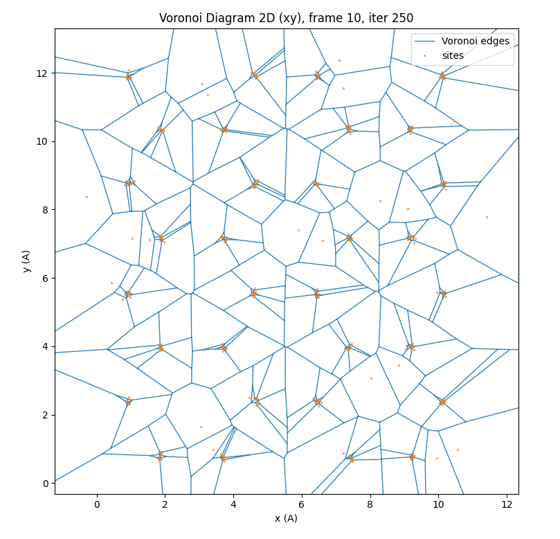
Figure: Sample an example 2D plot for the voronoi.
Common Runtime and Presentation Arguments
These are shared workflow-level CLI flags added before command-specific options, covering runtime context (engine/input/storage) and output presentation/export behavior.
Each command table above includes its shared and inherited options.